|
|
|
[*Back to home*](Home)
|
|
|
|
|
|
|
|
# Description of output files & folders
|
|
|
|
|
|
|
|
## Structure overview
|
|
|
|
|
|
|
|
The main output folder corresponds to the `-w` (or `--workdir`) specified for the creation of the [configuration file](usage/run_pipeline). If this option was not used, the main output folder defaults to a folder named "RESULTS" where the snakemake command was launched.
|
|
|
|
|
|
|
|
The output tree is as follows:
|
|
|
|
|
|
|
|
```sh
|
|
|
|
📦RESULTS # main output folder
|
|
|
|
┣ 📂TestProject # project folder (column 4 in samplesheet)
|
|
|
|
┃ ┣ 📂FASTQ # temporary folder for fastq files
|
|
|
|
┃ ┣ 📂FASTQC # FastQC results
|
|
|
|
┃ ┃ ┣ 📜sample1_fastqc.html
|
|
|
|
┃ ┃ ┣ 📜sample1_fastqc.zip
|
|
|
|
┃ ┃ ┣ ...
|
|
|
|
┃ ┣ 📂CUTADAPT # fastq files after cutadapt
|
|
|
|
┃ ┃ ┣ 📜sample1.fastq.gz
|
|
|
|
┃ ┃ ┣ 📜sample2.fastq.gz
|
|
|
|
┃ ┃ ┣ ...
|
|
|
|
┃ ┣ 📂MULTIQC # multiQC results
|
|
|
|
┃ ┃ ┣ 📂multiqc_data
|
|
|
|
┃ ┃ ┃ ┣ 📜multiqc.log
|
|
|
|
┃ ┃ ┃ ┣ 📜multiqc_data.json
|
|
|
|
┃ ┃ ┃ ┣ 📜multiqc_fastqc.txt
|
|
|
|
┃ ┃ ┃ ┣ 📜multiqc_general_stats.txt
|
|
|
|
┃ ┃ ┃ ┗ 📜multiqc_sources.txt
|
|
|
|
┃ ┃ ┗ 📜multiqc_report.html
|
|
|
|
┃ ┣ 📂ALIGNMENT # bam files after bwa alignment
|
|
|
|
┃ ┃ ┣ 📜sample1.bai
|
|
|
|
┃ ┃ ┣ 📜sample1.bam
|
|
|
|
┃ ┃ ┣ 📜sample2.bai
|
|
|
|
┃ ┃ ┣ 📜sample2.bam
|
|
|
|
┃ ┃ ┣ ...
|
|
|
|
┃ ┣ 📂EXPRESSION # primary analysis results
|
|
|
|
┃ ┃ ┣ 📜TestProject.all.log.dat
|
|
|
|
┃ ┃ ┣ 📜TestProject.all.refseq.total.dat
|
|
|
|
┃ ┃ ┣ 📜TestProject.all.refseq.umi.dat
|
|
|
|
┃ ┃ ┣ 📜TestProject.all.spike.total.dat
|
|
|
|
┃ ┃ ┣ 📜TestProject.all.spike.umi.dat
|
|
|
|
┃ ┃ ┣ 📜TestProject.all.unknown_list
|
|
|
|
┃ ┃ ┣ 📜TestProject.all.well_summary.dat
|
|
|
|
┃ ┃ ┣ 📜TestProject.all.well_summary.pdf
|
|
|
|
┃ ┃ ┣ 📜TestProject.unq.log.dat
|
|
|
|
┃ ┃ ┣ 📜TestProject.unq.refseq.total.dat
|
|
|
|
┃ ┃ ┣ 📜TestProject.unq.refseq.umi.dat
|
|
|
|
┃ ┃ ┣ 📜TestProject.unq.spike.total.dat
|
|
|
|
┃ ┃ ┣ 📜TestProject.unq.spike.umi.dat
|
|
|
|
┃ ┃ ┣ 📜TestProject.unq.unknown_list
|
|
|
|
┃ ┃ ┣ 📜TestProject.unq.well_summary.dat
|
|
|
|
┃ ┃ ┗ 📜TestProject.unq.well_summary.pdf
|
|
|
|
┃ ┣ 📂DE # secondary analysis results
|
|
|
|
┃ ┃ ┣ 📂cond1__vs__cond2 # comparisons results (1/3)
|
|
|
|
┃ ┃ ┃ ┣ 📜DEseqRes.tsv
|
|
|
|
┃ ┃ ┃ ┣ 📜DEseqResFiltered.tsv
|
|
|
|
┃ ┃ ┃ ┣ 📜MA-plot.png
|
|
|
|
┃ ┃ ┃ ┣ 📜Volcano-plot.png
|
|
|
|
┃ ┃ ┃ ┣ 📜annotGo.txt
|
|
|
|
┃ ┃ ┃ ┣ 📜annotKegg.txt
|
|
|
|
┃ ┃ ┃ ┣ 📜clustDEgene.pdf
|
|
|
|
┃ ┃ ┃ ┣ 📜clustDEgene.png
|
|
|
|
┃ ┃ ┃ ┣ 📜dotplotGO.png
|
|
|
|
┃ ┃ ┃ ┣ 📜dotplotKEGG.png
|
|
|
|
┃ ┃ ┃ ┣ 📜gseGo.txt
|
|
|
|
┃ ┃ ┃ ┣ 📜gseKegg.txt
|
|
|
|
┃ ┃ ┃ ┣ 📜stringDB-genes.txt
|
|
|
|
┃ ┃ ┃ ┗ 📜stringFunctionalEnrichment.tsv
|
|
|
|
┃ ┃ ┣ 📂cond1__vs__cond3 # comparisons results (2/3)
|
|
|
|
┃ ┃ ┃ ┣ 📜DEseqRes.tsv
|
|
|
|
┃ ┃ ┃ ┣ 📜DEseqRes.tsv
|
|
|
|
┃ ┃ ┃ ┣ ...
|
|
|
|
┃ ┃ ┣ 📂cond2__vs__cond3 # comparisons results (3/3)
|
|
|
|
┃ ┃ ┃ ┣ 📜DEseqRes.tsv
|
|
|
|
┃ ┃ ┃ ┣ 📜DEseqRes.tsv
|
|
|
|
┃ ┃ ┃ ┣ ...
|
|
|
|
┃ ┃ ┣ 📜HeatmapCorPearson.pdf
|
|
|
|
┃ ┃ ┣ 📜HeatmapCorPearson.png
|
|
|
|
┃ ┃ ┣ 📜NormAndPCA.pdf
|
|
|
|
┃ ┃ ┣ 📜PCA.png
|
|
|
|
┃ ┃ ┣ 📜SamplesAbstract.tsv
|
|
|
|
┃ ┃ ┣ 📜dds.RData
|
|
|
|
┃ ┃ ┣ 📜exprDatUPM.tsv
|
|
|
|
┃ ┃ ┣ 📜exprFiltered.tsv
|
|
|
|
┃ ┃ ┣ 📜exprNormalized.tsv
|
|
|
|
┃ ┃ ┣ 📜exprTransformed.tsv
|
|
|
|
┃ ┃ ┣ 📜heatmap.RData
|
|
|
|
┃ ┃ ┣ 📜normCountsDistri.png
|
|
|
|
┃ ┃ ┣ 📜samplesToKeep.txt
|
|
|
|
┃ ┃ ┣ 📜samplesToRemove.txt
|
|
|
|
┃ ┃ ┗ 📜sampletable.tsv
|
|
|
|
┃ ┣ 📂REPORT # necessary files for report (js, css, etc...)
|
|
|
|
┃ ┗ 📜report.html #### MAIN REPORT FOR PROJECT ####
|
|
|
|
┣ 📜RUNINFO.txt
|
|
|
|
┣ 📜config_used_in_analysis.json
|
|
|
|
┣ 📜unknown.fastq.gz
|
|
|
|
┣ 📂EXPRESSION # RUN primary analysis results (for stats only)
|
|
|
|
┃ ┣ 📜run.all.log.dat
|
|
|
|
┃ ┣ 📜run.all.well_summary.dat
|
|
|
|
┃ ┣ 📜run.all.well_summary.pdf
|
|
|
|
┃ ┣ 📜run.unq.log.dat
|
|
|
|
┃ ┣ 📜run.unq.well_summary.dat
|
|
|
|
┃ ┗ 📜run.unq.well_summary.pdf
|
|
|
|
┣ 📂MULTIQC # RUN multiQC results (for stats only)
|
|
|
|
┃ ┣ 📂multiqc_data
|
|
|
|
┃ ┃ ┣ 📜multiqc.log
|
|
|
|
┃ ┃ ┣ 📜multiqc_data.json
|
|
|
|
┃ ┃ ┣ 📜multiqc_fastqc.txt
|
|
|
|
┃ ┃ ┣ 📜multiqc_general_stats.txt
|
|
|
|
┃ ┃ ┗ 📜multiqc_sources.txt
|
|
|
|
┗ ┗ 📜multiqc_report.html
|
|
|
|
```
|
|
|
|
|
|
|
|
## The primary analysis results
|
|
|
|
|
|
|
|
```sh
|
|
|
|
📦RESULTS # main output folder
|
|
|
|
┣ 📂TestProject # project folder (column 4 in samplesheet)
|
|
|
|
```
|
|
|
|
|
|
|
|
One folder per project specified in the samplesheet is created. The project name in the dummy dataset is called **TestProject**. This folder contains all the results for this project.
|
|
|
|
|
|
|
|
```sh
|
|
|
|
📦RESULTS # main output folder
|
|
|
|
┣ 📂TestProject
|
|
|
|
┃ ┣ 📂FASTQ # temporary folder for fastq files
|
|
|
|
┃ ┣ 📂FASTQC # FastQC results
|
|
|
|
┃ ┃ ┣ 📜sample1_fastqc.html
|
|
|
|
┃ ┃ ┣ 📜sample1_fastqc.zip
|
|
|
|
┃ ┃ ┣ ...
|
|
|
|
┃ ┣ 📂CUTADAPT # fastq files after cutadapt
|
|
|
|
┃ ┃ ┣ 📜sample1.fastq.gz
|
|
|
|
┃ ┃ ┣ 📜sample2.fastq.gz
|
|
|
|
┃ ┃ ┣ ...
|
|
|
|
┃ ┣ 📂MULTIQC # multiQC results
|
|
|
|
┃ ┃ ┣ 📂multiqc_data
|
|
|
|
┃ ┃ ┃ ┣ 📜multiqc.log
|
|
|
|
┃ ┃ ┃ ┣ 📜multiqc_data.json
|
|
|
|
┃ ┃ ┃ ┣ 📜multiqc_fastqc.txt
|
|
|
|
┃ ┃ ┃ ┣ 📜multiqc_general_stats.txt
|
|
|
|
┃ ┃ ┃ ┗ 📜multiqc_sources.txt
|
|
|
|
┃ ┃ ┗ 📜multiqc_report.html
|
|
|
|
```
|
|
|
|
|
|
|
|
The demultiplexed fastq files are created in the **FASTQ** folder. Each fastq file is then processed by cutadapt in order to remove the poly A tails if necessary and is then moved to the **CUTADAPT** folder. Old fastq files are removed from the **FASTQ** folder. FastQC is then used on the fastq files. All results are stored in the **FASTQC** folder. Once all files processed, multiQC is used to compile the fastqc files. The resulting multiqc report, as well as the raw data are located in the **MULTIQC** folder.
|
|
|
|
|
|
|
|
```sh
|
|
|
|
📦RESULTS # main output folder
|
|
|
|
┣ 📂TestProject
|
|
|
|
┃ ┣ 📂ALIGNMENT # bam files after bwa alignment
|
|
|
|
┃ ┃ ┣ 📜sample1.bai
|
|
|
|
┃ ┃ ┣ 📜sample1.bam
|
|
|
|
┃ ┃ ┣ 📜sample2.bai
|
|
|
|
┃ ┃ ┣ 📜sample2.bam
|
|
|
|
┃ ┃ ┣ ...
|
|
|
|
```
|
|
|
|
|
|
|
|
Each fastq file is then aligned on the reference transcriptome using bwa algorithm. The resulting bam file, as well as its index (bai file), are located in the **ALIGNMENT** folder.
|
|
|
|
|
|
|
|
```sh
|
|
|
|
📦RESULTS # main output folder
|
|
|
|
┣ 📂TestProject
|
|
|
|
┃ ┣ 📂EXPRESSION # primary analysis results
|
|
|
|
┃ ┃ ┣ 📜TestProject.all.log.dat
|
|
|
|
┃ ┃ ┣ 📜TestProject.all.refseq.total.dat
|
|
|
|
┃ ┃ ┣ 📜TestProject.all.refseq.umi.dat
|
|
|
|
┃ ┃ ┣ 📜TestProject.all.spike.total.dat
|
|
|
|
┃ ┃ ┣ 📜TestProject.all.spike.umi.dat
|
|
|
|
┃ ┃ ┣ 📜TestProject.all.unknown_list
|
|
|
|
┃ ┃ ┣ 📜TestProject.all.well_summary.dat
|
|
|
|
┃ ┃ ┣ 📜TestProject.all.well_summary.pdf
|
|
|
|
┃ ┃ ┣ 📜TestProject.unq.log.dat
|
|
|
|
┃ ┃ ┣ 📜TestProject.unq.refseq.total.dat
|
|
|
|
┃ ┃ ┣ 📜TestProject.unq.refseq.umi.dat
|
|
|
|
┃ ┃ ┣ 📜TestProject.unq.spike.total.dat
|
|
|
|
┃ ┃ ┣ 📜TestProject.unq.spike.umi.dat
|
|
|
|
┃ ┃ ┣ 📜TestProject.unq.unknown_list
|
|
|
|
┃ ┃ ┣ 📜TestProject.unq.well_summary.dat
|
|
|
|
┃ ┃ ┗ 📜TestProject.unq.well_summary.pdf
|
|
|
|
```
|
|
|
|
|
|
|
|
A python script is used to count the number of reads aligned on every gene for all samples. The results of this script are located in the **EXPRESSION** folder.
|
|
|
|
|
|
|
|
The name of the files start with the name of the project, here "TestProject".
|
|
|
|
The second part is either "all" or "unq":
|
|
|
|
- "all" counts reads that have aligned on multiple genes. The read count is assigned to the gene defined as the primary alignement in the bam files.
|
|
|
|
- "unq" counts only the reads which align on one gene. Reads can align on multiple transcripts but of only one gene.
|
|
|
|
|
|
|
|
The third part of the name defines the informations to be fount:
|
|
|
|
- "log" is a summary of the counts for the whole run.
|
|
|
|
- "refseq" is the expression matrix. It is there that you will find all counts for each sample and for each gene.
|
|
|
|
- "spike" is the count matrix of the spike-in. It is there for legacy reasons and is not used in our implementation of the technique.
|
|
|
|
- "unknown_list" is the list of the tracks present in the fasta file (ie, the list of transcript) which are not assigned to a gene in the sym2ref file (ie, no annotation).
|
|
|
|
- "well_summary" is a summary of the counts for each sample.
|
|
|
|
|
|
|
|
The fourth part of the name, only found in "refseq" and "spike" files can either be "total" or "umi":
|
|
|
|
- "total" is the number of total reads of the counts without taking into account the UMIs. Counts can be artificially increased by the PCR steps of the technique.
|
|
|
|
- "umi" is the number of unique molecules of RNA, this taking into account the UMIs for each read. If two reads of the same sample map to the same gene and have the same UMI, it will only be counted for 1.
|
|
|
|
|
|
|
|
**Thus, the expression matrix usually used for secondary analysis is "XXX.unq.refseq.umi.dat"**
|
|
|
|
|
|
|
|

|
|
|
|
|
|
|
|
## The secondary analysis results
|
|
|
|
|
|
|
|
```sh
|
|
|
|
📦RESULTS # main output folder
|
|
|
|
┣ 📂TestProject
|
|
|
|
┃ ┣ 📂DE # secondary analysis results
|
|
|
|
┃ ┃ ┣ 📂cond1__vs__cond2 # comparisons results (1/3)
|
|
|
|
┃ ┃ ┃ ┣ 📜DEseqRes.tsv
|
|
|
|
┃ ┃ ┃ ┣ 📜DEseqResFiltered.tsv
|
|
|
|
┃ ┃ ┃ ┣ 📜MA-plot.png
|
|
|
|
┃ ┃ ┃ ┣ 📜Volcano-plot.png
|
|
|
|
┃ ┃ ┃ ┣ 📜annotGo.txt
|
|
|
|
┃ ┃ ┃ ┣ 📜annotKegg.txt
|
|
|
|
┃ ┃ ┃ ┣ 📜clustDEgene.pdf
|
|
|
|
┃ ┃ ┃ ┣ 📜clustDEgene.png
|
|
|
|
┃ ┃ ┃ ┣ 📜dotplotGO.png
|
|
|
|
┃ ┃ ┃ ┣ 📜dotplotKEGG.png
|
|
|
|
┃ ┃ ┃ ┣ 📜gseGo.txt
|
|
|
|
┃ ┃ ┃ ┣ 📜gseKegg.txt
|
|
|
|
┃ ┃ ┃ ┣ 📜stringDB-genes.txt
|
|
|
|
┃ ┃ ┃ ┗ 📜stringFunctionalEnrichment.tsv
|
|
|
|
┃ ┃ ┣ 📂cond1__vs__cond3 # comparisons results (2/3)
|
|
|
|
┃ ┃ ┃ ┣ 📜DEseqRes.tsv
|
|
|
|
┃ ┃ ┃ ┣ 📜DEseqRes.tsv
|
|
|
|
┃ ┃ ┃ ┣ ...
|
|
|
|
┃ ┃ ┣ 📂cond2__vs__cond3 # comparisons results (3/3)
|
|
|
|
┃ ┃ ┃ ┣ 📜DEseqRes.tsv
|
|
|
|
┃ ┃ ┃ ┣ 📜DEseqRes.tsv
|
|
|
|
┃ ┃ ┃ ┣ ...
|
|
|
|
┃ ┃ ┣ 📜HeatmapCorPearson.pdf
|
|
|
|
┃ ┃ ┣ 📜HeatmapCorPearson.png
|
|
|
|
┃ ┃ ┣ 📜NormAndPCA.pdf
|
|
|
|
┃ ┃ ┣ 📜PCA.png
|
|
|
|
┃ ┃ ┣ 📜SamplesAbstract.tsv
|
|
|
|
┃ ┃ ┣ 📜dds.RData
|
|
|
|
┃ ┃ ┣ 📜exprDatUPM.tsv
|
|
|
|
┃ ┃ ┣ 📜exprFiltered.tsv
|
|
|
|
┃ ┃ ┣ 📜exprNormalized.tsv
|
|
|
|
┃ ┃ ┣ 📜exprTransformed.tsv
|
|
|
|
┃ ┃ ┣ 📜heatmap.RData
|
|
|
|
┃ ┃ ┣ 📜normCountsDistri.png
|
|
|
|
┃ ┃ ┣ 📜samplesToKeep.txt
|
|
|
|
┃ ┃ ┣ 📜samplesToRemove.txt
|
|
|
|
┃ ┃ ┗ 📜sampletable.tsv
|
|
|
|
┃ ┣ 📂REPORT # necessary files for report (js, css, etc...)
|
|
|
|
┃ ┗ 📜report.html #### MAIN REPORT FOR PROJECT ####
|
|
|
|
```
|
|
|
|
|
|
|
|
In the **DE** (stands for **D**ifferential **E**xpression) folder, you will find the results of the comparisons between conditions.
|
|
|
|
|
|
|
|
In the main folder are located the files common to all comparisons. This is a description of these files in the order that they will be created by the pipeline:
|
|
|
|
|
|
|
|
- "exprFiltered.tsv" : expression matrix where
|
|
|
|
- samples are removed according to the thresholds specified (defaults to 200k UMIs and 50k genes detected)
|
|
|
|
- genes will be removed in not expressed in at least the minimum number of samples in a condition. For example, if there are only three samples in condition X, then every gene must be expressed in at least three samples.
|
|
|
|
- "samplesToKeep.txt","samplesToRemove.txt" : names of the samples under the thresholds specified.
|
|
|
|
- "exprNormalized.tsv" : expression matrix normalized by deseq2 method. If you're not familiar with this normalization method, you can have a look at the very well explained [StatQuest deseq2 library normalization](https://www.youtube.com/watch?v=UFB993xufUU) video.
|
|
|
|
- "exprTransformed.tsv" : logged expression matrix made for visualization.
|
|
|
|
- "exprDatUPM.tsv" : expression matrix normalized by a simple method UMIs Per Million.
|
|
|
|
- "SamplesAbstract.tsv", "sampletable.tsv" : helper files for deseq2.
|
|
|
|
- "dds.RData", "heatmap.RData" : R data files for reuse in further scripts.
|
|
|
|
- "normCountsDistri.png" : Distribution of the normalized counts.
|
|
|
|
- "HeatmapCorPearson.png" : Headmap of the correlation between samples.
|
|
|
|
- "PCA.png" : Principle component analysis.
|
|
|
|
|
|
|
|

|
|
|
|
|
|
|
|
For each comparisons specified in *[the comparisons file](usage/inputs#compFile)*, a folder named **condition1__vs__condition2** is created. All files within this folder refers to this comparison only:
|
|
|
|
|
|
|
|
- "DEseqRes.tsv" : results of deseq2. Each line is the result of the statistical test determining if the gene is differentially expressed or not.
|
|
|
|
- "DEseqResFiltered.tsv" : same as above but only on genes considered differentially expressed according to the threshold of adjusted p-value (0.05) and logFC (0.58).
|
|
|
|
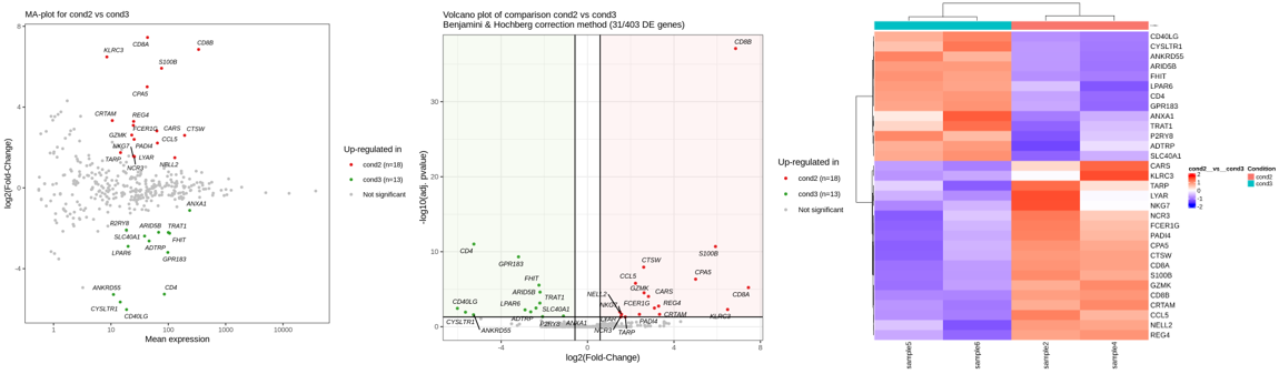
- "MA-plot.png", "Volcano-plot.png" : representations of the differentially expressed genes.
|
|
|
|
- "clustDEgene.png" : heatmap of the differentially expressed genes for the samples included in the comparison only.
|
|
|
|
- "clustDEgene.pdf" : same as above enriched with a heatmap of the differentially expressed genes for all samples of the project.
|
|
|
|
|
|
|
|
|
|
|
|
|
|
|
|
The other files of this folder are results of tertiary analysis tools. They give an insight on the meaning of the list of differentially expressed genes.
|
|
|
|
|
|
|
|
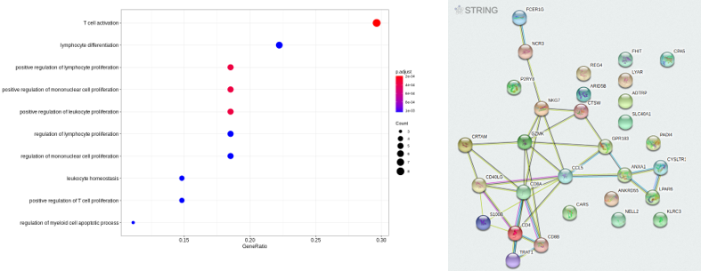
- "annotGo.txt", "annotKegg.txt" : over-representation analysis (ORA) of Gene Ontology and Kegg Pathways respectively. This is text table listing all ontologies and pathways with their adjusted p-values.
|
|
|
|
- "dotplotGO.png", "dotplotKEGG.png" : graphical representation of the ORA results above.
|
|
|
|
- "gseGo.txt", "gseKegg.txt" : Gene Set Enrichment Analysis (GSEA) results for Gene Ontology and Kegg Pathways. You can find all about GSEA analysis on the [Broad Institut GSEA page](https://www.gsea-msigdb.org/gsea/index.jsp).
|
|
|
|
- "stringFunctionalEnrichment.tsv" : ORA analysis from the [STRING-DB](https://string-db.org/) database.
|
|
|
|
|
|
|
|
 |
|
|
\ No newline at end of file |